BGGN 213 Spring 2019 Classwork
https://androidpcguy.github.io/bggn213/
Class 14: RNAseq analysis
Akshara Balachandra 5/17/2019
Library imports…
library(DESeq2)
## Loading required package: S4Vectors

## Loading required package: stats4

## Loading required package: BiocGenerics

## Loading required package: parallel

##
## Attaching package: 'BiocGenerics'

## The following objects are masked from 'package:parallel':
##
##     clusterApply, clusterApplyLB, clusterCall, clusterEvalQ,
##     clusterExport, clusterMap, parApply, parCapply, parLapply,
##     parLapplyLB, parRapply, parSapply, parSapplyLB

## The following objects are masked from 'package:stats':
##
##     IQR, mad, sd, var, xtabs

## The following objects are masked from 'package:base':
##
##     anyDuplicated, append, as.data.frame, basename, cbind,
##     colnames, dirname, do.call, duplicated, eval, evalq, Filter,
##     Find, get, grep, grepl, intersect, is.unsorted, lapply, Map,
##     mapply, match, mget, order, paste, pmax, pmax.int, pmin,
##     pmin.int, Position, rank, rbind, Reduce, rownames, sapply,
##     setdiff, sort, table, tapply, union, unique, unsplit, which,
##     which.max, which.min

##
## Attaching package: 'S4Vectors'

## The following object is masked from 'package:base':
##
##     expand.grid

## Loading required package: IRanges

## Loading required package: GenomicRanges

## Loading required package: GenomeInfoDb

## Loading required package: SummarizedExperiment

## Loading required package: Biobase

## Welcome to Bioconductor
##
##     Vignettes contain introductory material; view with
##     'browseVignettes()'. To cite Bioconductor, see
##     'citation("Biobase")', and for packages 'citation("pkgname")'.

## Loading required package: DelayedArray

## Loading required package: matrixStats

##
## Attaching package: 'matrixStats'

## The following objects are masked from 'package:Biobase':
##
##     anyMissing, rowMedians

## Loading required package: BiocParallel

##
## Attaching package: 'DelayedArray'

## The following objects are masked from 'package:matrixStats':
##
##     colMaxs, colMins, colRanges, rowMaxs, rowMins, rowRanges

## The following objects are masked from 'package:base':
##
##     aperm, apply, rowsum

## Registered S3 methods overwritten by 'ggplot2':
##   method         from
##   [.quosures     rlang
##   c.quosures     rlang
##   print.quosures rlang
library(tibble)
library(dplyr)
##
## Attaching package: 'dplyr'

## The following object is masked from 'package:matrixStats':
##
##     count

## The following object is masked from 'package:Biobase':
##
##     combine

## The following objects are masked from 'package:GenomicRanges':
##
##     intersect, setdiff, union

## The following object is masked from 'package:GenomeInfoDb':
##
##     intersect

## The following objects are masked from 'package:IRanges':
##
##     collapse, desc, intersect, setdiff, slice, union

## The following objects are masked from 'package:S4Vectors':
##
##     first, intersect, rename, setdiff, setequal, union

## The following objects are masked from 'package:BiocGenerics':
##
##     combine, intersect, setdiff, union

## The following objects are masked from 'package:stats':
##
##     filter, lag

## The following objects are masked from 'package:base':
##
##     intersect, setdiff, setequal, union
Read count data and metadata…
counts <- read.csv('data/airway_scaledcounts.csv', stringsAsFactors = F, row.names = 1)
metadata <- read.csv('data/airway_metadata.csv', stringsAsFactors = F)

#counts
#metadata

nrow(counts)
## [1] 38694
sum(metadata$dex == 'control')
## [1] 4
Q1: There are 38694 genes in the dataset. Q2: There are 4 control cell lines
Toy differential gene expression
control.cells <- metadata$id[metadata$dex == 'control']
treated.cells <- metadata$id[metadata$dex == 'treated']

control.sub <- subset(counts, select = control.cells)
treated.sub <- subset(counts, select = treated.cells)

control.means <- apply(control.sub, 1, mean)
treated.means <- apply(treated.sub, 1, mean)
control.mean <- sum(control.means)
treated.mean <- sum(treated.means)

mean.counts <- data.frame(control.means, treated.means)

print(paste('Control mean', round(control.mean)))
## [1] "Control mean 23005324"
print(paste('Treated mean', round(treated.mean)))
## [1] "Treated mean 22196524"
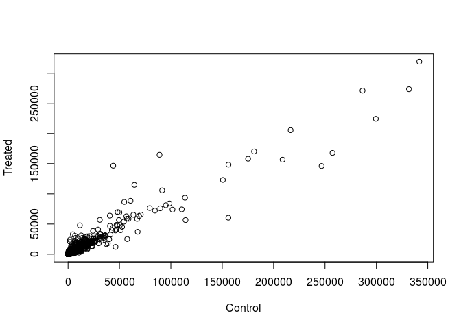
Scatter plot of means of controls vs treated…
plot(control.means, treated.means, xlab = 'Control',
     ylab = 'Treated')
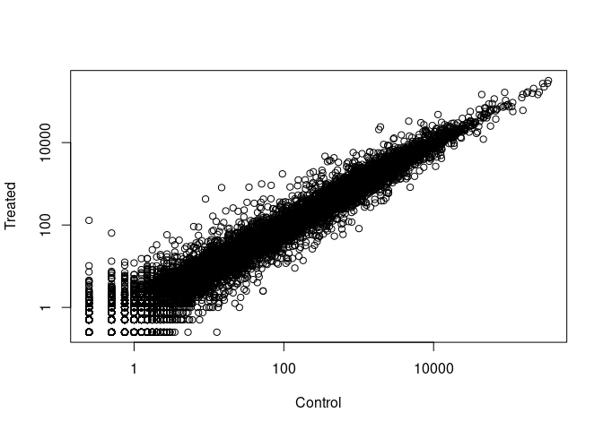
Plot with log scale…
plot(control.means, treated.means, xlab = 'Control',
     ylab = 'Treated', log = 'xy')
## Warning in xy.coords(x, y, xlabel, ylabel, log): 15032 x values <= 0
## omitted from logarithmic plot

## Warning in xy.coords(x, y, xlabel, ylabel, log): 15281 y values <= 0
## omitted from logarithmic plot
Let’s combine the control and treated means and calculate log2 fold change…
mean.counts <- data.frame(control.means, treated.means,
                          row.names = row.names(counts))

mean.counts$log2foldchange <- log((mean.counts$treated.means/mean.counts$control.means),
                                  base = 2)

head(mean.counts)
##                 control.means treated.means log2foldchange
## ENSG00000000003        900.75        658.00    -0.45303916
## ENSG00000000005          0.00          0.00            NaN
## ENSG00000000419        520.50        546.00     0.06900279
## ENSG00000000457        339.75        316.50    -0.10226805
## ENSG00000000460         97.25         78.75    -0.30441833
## ENSG00000000938          0.75          0.00           -Inf
Let’s filter out the genes that had 0 expression…
mean.counts <- mean.counts %>% rownames_to_column('gene') %>%
  filter(is.finite(log2foldchange)) %>% column_to_rownames('gene')
head(mean.counts)
##                 control.means treated.means log2foldchange
## ENSG00000000003        900.75        658.00    -0.45303916
## ENSG00000000419        520.50        546.00     0.06900279
## ENSG00000000457        339.75        316.50    -0.10226805
## ENSG00000000460         97.25         78.75    -0.30441833
## ENSG00000000971       5219.00       6687.50     0.35769358
## ENSG00000001036       2327.00       1785.75    -0.38194109
Let’s figure out now how many genes are upregulated and downregulated after adding the treatment
up.regulated <- mean.counts %>% rownames_to_column('gene') %>%
  filter(log2foldchange > 2) %>% column_to_rownames('gene')

down.regulated <- mean.counts %>% rownames_to_column('gene') %>%
  filter(log2foldchange < -2) %>% column_to_rownames('gene')

head(up.regulated)
##                 control.means treated.means log2foldchange
## ENSG00000004799        270.50       1429.25       2.401558
## ENSG00000006788          2.75         19.75       2.844349
## ENSG00000008438          0.50          2.75       2.459432
## ENSG00000011677          0.50          2.25       2.169925
## ENSG00000015413          0.50          3.00       2.584963
## ENSG00000015592          0.50          2.25       2.169925
head(down.regulated)
##                 control.means treated.means log2foldchange
## ENSG00000015520         32.00          6.00      -2.415037
## ENSG00000019186         26.50          1.75      -3.920566
## ENSG00000025423        295.00         54.25      -2.443020
## ENSG00000028277         88.25         22.00      -2.004093
## ENSG00000029559          1.25          0.25      -2.321928
## ENSG00000049246        405.00         93.00      -2.122619
print(paste('There are', nrow(up.regulated), 'upregulated genes relative to control'))
## [1] "There are 250 upregulated genes relative to control"
print(paste('There are', nrow(down.regulated), 'downregulated genes relative to control'))
## [1] "There are 367 downregulated genes relative to control"
Adding annotation data
Merge mean.counts with annotation data…
# read in annotations
annot <- read.csv('data/annotables_grch38.csv',
                  stringsAsFactors = F,
                  row.names = NULL)

# filter out duplicate entries
annot <- annot[!duplicated(annot$ensgene),]

row.names(annot) <- NULL

annot <- annot %>% column_to_rownames('ensgene')
head(annot)
##                 entrez   symbol chr     start       end strand
## ENSG00000000003   7105   TSPAN6   X 100627109 100639991     -1
## ENSG00000000005  64102     TNMD   X 100584802 100599885      1
## ENSG00000000419   8813     DPM1  20  50934867  50958555     -1
## ENSG00000000457  57147    SCYL3   1 169849631 169894267     -1
## ENSG00000000460  55732 C1orf112   1 169662007 169854080      1
## ENSG00000000938   2268      FGR   1  27612064  27635277     -1
##                        biotype
## ENSG00000000003 protein_coding
## ENSG00000000005 protein_coding
## ENSG00000000419 protein_coding
## ENSG00000000457 protein_coding
## ENSG00000000460 protein_coding
## ENSG00000000938 protein_coding
##                                                                                                                description
## ENSG00000000003                                                          tetraspanin 6 [Source:HGNC Symbol;Acc:HGNC:11858]
## ENSG00000000005                                                            tenomodulin [Source:HGNC Symbol;Acc:HGNC:17757]
## ENSG00000000419 dolichyl-phosphate mannosyltransferase polypeptide 1, catalytic subunit [Source:HGNC Symbol;Acc:HGNC:3005]
## ENSG00000000457                                               SCY1-like, kinase-like 3 [Source:HGNC Symbol;Acc:HGNC:19285]
## ENSG00000000460                                    chromosome 1 open reading frame 112 [Source:HGNC Symbol;Acc:HGNC:25565]
## ENSG00000000938                          FGR proto-oncogene, Src family tyrosine kinase [Source:HGNC Symbol;Acc:HGNC:3697]
Merge annotation with colmeans now.
mean.counts.meta <- merge(x = mean.counts,
                          y = annot,
                          by = 0) %>% # by = 0 (rownames)
  column_to_rownames('Row.names')

head(mean.counts.meta)
##                 control.means treated.means log2foldchange entrez   symbol
## ENSG00000000003        900.75        658.00    -0.45303916   7105   TSPAN6
## ENSG00000000419        520.50        546.00     0.06900279   8813     DPM1
## ENSG00000000457        339.75        316.50    -0.10226805  57147    SCYL3
## ENSG00000000460         97.25         78.75    -0.30441833  55732 C1orf112
## ENSG00000000971       5219.00       6687.50     0.35769358   3075      CFH
## ENSG00000001036       2327.00       1785.75    -0.38194109   2519    FUCA2
##                 chr     start       end strand        biotype
## ENSG00000000003   X 100627109 100639991     -1 protein_coding
## ENSG00000000419  20  50934867  50958555     -1 protein_coding
## ENSG00000000457   1 169849631 169894267     -1 protein_coding
## ENSG00000000460   1 169662007 169854080      1 protein_coding
## ENSG00000000971   1 196651878 196747504      1 protein_coding
## ENSG00000001036   6 143494811 143511690     -1 protein_coding
##                                                                                                                description
## ENSG00000000003                                                          tetraspanin 6 [Source:HGNC Symbol;Acc:HGNC:11858]
## ENSG00000000419 dolichyl-phosphate mannosyltransferase polypeptide 1, catalytic subunit [Source:HGNC Symbol;Acc:HGNC:3005]
## ENSG00000000457                                               SCY1-like, kinase-like 3 [Source:HGNC Symbol;Acc:HGNC:19285]
## ENSG00000000460                                    chromosome 1 open reading frame 112 [Source:HGNC Symbol;Acc:HGNC:25565]
## ENSG00000000971                                                     complement factor H [Source:HGNC Symbol;Acc:HGNC:4883]
## ENSG00000001036                                          fucosidase, alpha-L- 2, plasma [Source:HGNC Symbol;Acc:HGNC:4008]
Read in annotation package for homo sapiens (humans)
library('AnnotationDbi')
##
## Attaching package: 'AnnotationDbi'

## The following object is masked from 'package:dplyr':
##
##     select
library('org.Hs.eg.db')
##
columns(org.Hs.eg.db)
##  [1] "ACCNUM"       "ALIAS"        "ENSEMBL"      "ENSEMBLPROT"
##  [5] "ENSEMBLTRANS" "ENTREZID"     "ENZYME"       "EVIDENCE"
##  [9] "EVIDENCEALL"  "GENENAME"     "GO"           "GOALL"
## [13] "IPI"          "MAP"          "OMIM"         "ONTOLOGY"
## [17] "ONTOLOGYALL"  "PATH"         "PFAM"         "PMID"
## [21] "PROSITE"      "REFSEQ"       "SYMBOL"       "UCSCKG"
## [25] "UNIGENE"      "UNIPROT"
Add information to the counts data frame…
mean.counts$symbol <- mapIds(org.Hs.eg.db, keytype = 'ENSEMBL',
       keys = row.names(mean.counts),
       column = 'SYMBOL',
       multiVals = 'first')
## 'select()' returned 1:many mapping between keys and columns
mean.counts$entrez <- mapIds(org.Hs.eg.db, keytype = 'ENSEMBL',
       keys = row.names(mean.counts),
       column = 'ENTREZID',
       multiVals = 'first')
## 'select()' returned 1:many mapping between keys and columns
mean.counts$uniprot <- mapIds(org.Hs.eg.db, keytype = 'ENSEMBL',
       keys = row.names(mean.counts),
       column = 'UNIPROT',
       multiVals = 'first')
## 'select()' returned 1:many mapping between keys and columns
head(mean.counts)
##                 control.means treated.means log2foldchange   symbol entrez
## ENSG00000000003        900.75        658.00    -0.45303916   TSPAN6   7105
## ENSG00000000419        520.50        546.00     0.06900279     DPM1   8813
## ENSG00000000457        339.75        316.50    -0.10226805    SCYL3  57147
## ENSG00000000460         97.25         78.75    -0.30441833 C1orf112  55732
## ENSG00000000971       5219.00       6687.50     0.35769358      CFH   3075
## ENSG00000001036       2327.00       1785.75    -0.38194109    FUCA2   2519
##                    uniprot
## ENSG00000000003 A0A024RCI0
## ENSG00000000419     O60762
## ENSG00000000457     Q8IZE3
## ENSG00000000460 A0A024R922
## ENSG00000000971 A0A024R962
## ENSG00000001036     Q9BTY2
Q12:
head(mean.counts[row.names(up.regulated),])
##                 control.means treated.means log2foldchange  symbol entrez
## ENSG00000004799        270.50       1429.25       2.401558    PDK4   5166
## ENSG00000006788          2.75         19.75       2.844349   MYH13   8735
## ENSG00000008438          0.50          2.75       2.459432 PGLYRP1   8993
## ENSG00000011677          0.50          2.25       2.169925  GABRA3   2556
## ENSG00000015413          0.50          3.00       2.584963   DPEP1   1800
## ENSG00000015592          0.50          2.25       2.169925   STMN4  81551
##                    uniprot
## ENSG00000004799     A4D1H4
## ENSG00000006788     Q9UKX3
## ENSG00000008438     O75594
## ENSG00000011677     P34903
## ENSG00000015413 A0A140VJI3
## ENSG00000015592     Q9H169
head(mean.counts[row.names(down.regulated),])
##                 control.means treated.means log2foldchange  symbol entrez
## ENSG00000015520         32.00          6.00      -2.415037  NPC1L1  29881
## ENSG00000019186         26.50          1.75      -3.920566 CYP24A1   1591
## ENSG00000025423        295.00         54.25      -2.443020 HSD17B6   8630
## ENSG00000028277         88.25         22.00      -2.004093  POU2F2   5452
## ENSG00000029559          1.25          0.25      -2.321928    IBSP   3381
## ENSG00000049246        405.00         93.00      -2.122619    PER3   8863
##                    uniprot
## ENSG00000015520 A0A0C4DFX6
## ENSG00000019186     Q07973
## ENSG00000025423 A0A024RB43
## ENSG00000028277     P09086
## ENSG00000029559     P21815
## ENSG00000049246 A0A087WV69
I would not trust these results because we don’t know if these results are true or just false positives.
DESeq2 analysis
counts <- counts %>% rownames_to_column('ensgene')
dds <- DESeqDataSetFromMatrix(countData = counts,colData = metadata, design=~dex,
                              tidy = TRUE)
## converting counts to integer mode

## Warning in DESeqDataSet(se, design = design, ignoreRank): some variables in
## design formula are characters, converting to factors
dds
## class: DESeqDataSet
## dim: 38694 8
## metadata(1): version
## assays(1): counts
## rownames(38694): ENSG00000000003 ENSG00000000005 ...
##   ENSG00000283120 ENSG00000283123
## rowData names(0):
## colnames(8): SRR1039508 SRR1039509 ... SRR1039520 SRR1039521
## colData names(4): id dex celltype geo_id
dds <- DESeq(dds)
## estimating size factors

## estimating dispersions

## gene-wise dispersion estimates

## mean-dispersion relationship

## final dispersion estimates

## fitting model and testing
Get the results for threshold of log2foldchange of +/- 2, alpha level of 0.05…
res <- results(dds)
head(as.data.frame(res))
##                    baseMean log2FoldChange     lfcSE       stat     pvalue
## ENSG00000000003 747.1941954    -0.35070302 0.1682457 -2.0844697 0.03711747
## ENSG00000000005   0.0000000             NA        NA         NA         NA
## ENSG00000000419 520.1341601     0.20610777 0.1010592  2.0394752 0.04140263
## ENSG00000000457 322.6648439     0.02452695 0.1451451  0.1689823 0.86581056
## ENSG00000000460  87.6826252    -0.14714205 0.2570073 -0.5725210 0.56696907
## ENSG00000000938   0.3191666    -1.73228897 3.4936010 -0.4958463 0.62000288
##                      padj
## ENSG00000000003 0.1630348
## ENSG00000000005        NA
## ENSG00000000419 0.1760317
## ENSG00000000457 0.9616942
## ENSG00000000460 0.8158486
## ENSG00000000938        NA
summary(res)
##
## out of 25258 with nonzero total read count
## adjusted p-value < 0.1
## LFC > 0 (up)       : 1563, 6.2%
## LFC < 0 (down)     : 1188, 4.7%
## outliers [1]       : 142, 0.56%
## low counts [2]     : 9971, 39%
## (mean count < 10)
## [1] see 'cooksCutoff' argument of ?results
## [2] see 'independentFiltering' argument of ?results
Significance of 0.01…
resSig01 <- results(dds, alpha = .01)
#head(as.data.frame(resSig01))

summary(resSig01)
##
## out of 25258 with nonzero total read count
## adjusted p-value < 0.01
## LFC > 0 (up)       : 850, 3.4%
## LFC < 0 (down)     : 581, 2.3%
## outliers [1]       : 142, 0.56%
## low counts [2]     : 9033, 36%
## (mean count < 6)
## [1] see 'cooksCutoff' argument of ?results
## [2] see 'independentFiltering' argument of ?results
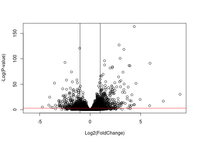
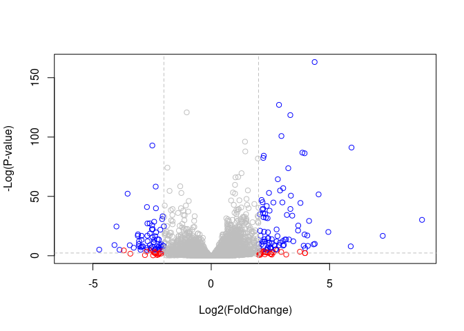
Visualize
plot( res$log2FoldChange,  -log(res$padj),
      xlab="Log2(FoldChange)",
      ylab="-Log(P-value)")

abline(h = -log(0.05), col = 'red')
abline(v = log(2, base = 2))
abline(v = -log(2, base = 2))
mycols <- rep("gray", nrow(res))
mycols[ abs(res$log2FoldChange) > 2 ]  <- "red"

inds <- (res$padj < 0.01) & (abs(res$log2FoldChange) > 2 )
mycols[ inds ] <- "blue"

# Volcano plot with custom colors
plot( res$log2FoldChange,  -log(res$padj),
 col=mycols, ylab="-Log(P-value)", xlab="Log2(FoldChange)" )

# Cut-off lines
abline(v=c(-2,2), col="gray", lty=2)
abline(h=-log(0.1), col="gray", lty=2)
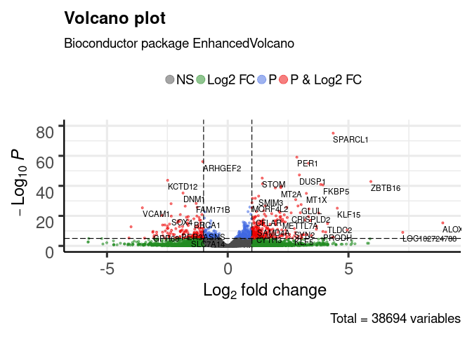
We can use the enhanced volcano plotting functions in bioconductor. First, let’s add the annotations.
x <- as.data.frame(res)
x$symbol <- mapIds(org.Hs.eg.db,
                   keys=row.names(x),
                   keytype="ENSEMBL",
                   column="SYMBOL",
                   multiVals="first")
## 'select()' returned 1:many mapping between keys and columns
library(EnhancedVolcano)
## Loading required package: ggplot2

## Loading required package: ggrepel
EnhancedVolcano(x, lab = x$symbol, x = 'log2FoldChange', y = 'pvalue')