BGGN 213 Spring 2019 Classwork
https://androidpcguy.github.io/bggn213/
Class 17 - Network Analysis
Akshara Balachandra 5/29/2019
Set up Cytoscape and R connection
Load the required packages RCy3 from bioconductor and igraph from CRAN.
library(RCy3)
## Registered S3 method overwritten by 'R.oo':
##   method        from
##   throw.default R.methodsS3
library(igraph)
##
## Attaching package: 'igraph'

## The following objects are masked from 'package:stats':
##
##     decompose, spectrum

## The following object is masked from 'package:base':
##
##     union
Check connection to Cytoscape…
cytoscapePing()
## [1] "You are connected to Cytoscape!"
Make a simple graph
g <- makeSimpleIgraph()
createNetworkFromIgraph(g,"myGraph")
## Loading data...
## Applying default style...
## Applying preferred layout...

## networkSUID
##        7763
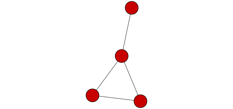
Include the graph in this report.
fig <- exportImage(filename="demo", type="png", height=350)
## Warning: This file already exists. A Cytoscape popup
##                 will be generated to confirm overwrite.
knitr::include_graphics('demo.png')
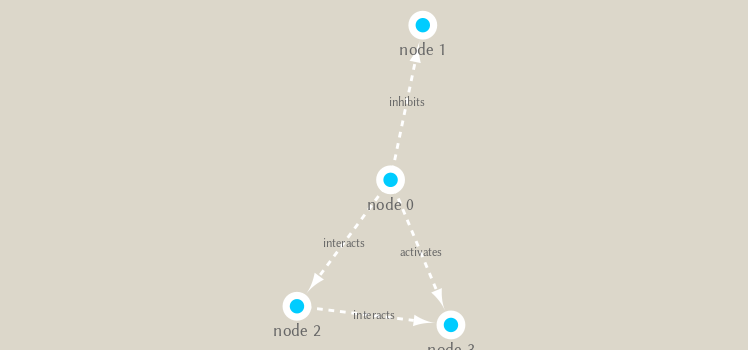
Change the visual style…
setVisualStyle("Marquee")
##                 message
## "Visual Style applied."
fig <- exportImage(filename="demo_marquee", type="png", height=350)
## Warning: This file already exists. A Cytoscape popup
##                 will be generated to confirm overwrite.
knitr::include_graphics("./demo_marquee.png")
Actual metagenomics data
Read the data….
prok_vir_cor <- read.delim("./data/virus_prok_cor_abundant.tsv", stringsAsFactors = FALSE)

## Have a peak at the first 6 rows
head(prok_vir_cor)
##       Var1          Var2    weight
## 1  ph_1061 AACY020068177 0.8555342
## 2  ph_1258 AACY020207233 0.8055750
## 3  ph_3164 AACY020207233 0.8122517
## 4  ph_1033 AACY020255495 0.8487498
## 5 ph_10996 AACY020255495 0.8734617
## 6 ph_11038 AACY020255495 0.8740782
Create the graph
g <- graph.data.frame(prok_vir_cor, directed = F)
class(g)
## [1] "igraph"
g
## IGRAPH ede583f UNW- 845 1544 --
## + attr: name (v/c), weight (e/n)
## + edges from ede583f (vertex names):
##  [1] ph_1061 --AACY020068177 ph_1258 --AACY020207233
##  [3] ph_3164 --AACY020207233 ph_1033 --AACY020255495
##  [5] ph_10996--AACY020255495 ph_11038--AACY020255495
##  [7] ph_11040--AACY020255495 ph_11048--AACY020255495
##  [9] ph_11096--AACY020255495 ph_1113 --AACY020255495
## [11] ph_1208 --AACY020255495 ph_13207--AACY020255495
## [13] ph_1346 --AACY020255495 ph_14679--AACY020255495
## [15] ph_1572 --AACY020255495 ph_16045--AACY020255495
## + ... omitted several edges
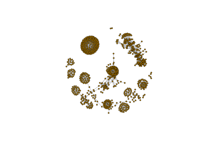
Plot it
plot(g, vertex.label = NA)
Make the nodes smaller
plot(g, vertex.label = NA, vertex.size = 3)
Network queries
V(g)
## + 845/845 vertices, named, from ede583f:
##   [1] ph_1061       ph_1258       ph_3164       ph_1033       ph_10996
##   [6] ph_11038      ph_11040      ph_11048      ph_11096      ph_1113
##  [11] ph_1208       ph_13207      ph_1346       ph_14679      ph_1572
##  [16] ph_16045      ph_1909       ph_1918       ph_19894      ph_2117
##  [21] ph_2231       ph_2363       ph_276        ph_2775       ph_2798
##  [26] ph_3217       ph_3336       ph_3493       ph_3541       ph_3892
##  [31] ph_4194       ph_4602       ph_4678       ph_484        ph_4993
##  [36] ph_4999       ph_5001       ph_5010       ph_5286       ph_5287
##  [41] ph_5302       ph_5321       ph_5643       ph_6441       ph_654
##  [46] ph_6954       ph_7389       ph_7920       ph_8039       ph_8695
## + ... omitted several vertices
E(g)
## + 1544/1544 edges from ede583f (vertex names):
##  [1] ph_1061 --AACY020068177 ph_1258 --AACY020207233
##  [3] ph_3164 --AACY020207233 ph_1033 --AACY020255495
##  [5] ph_10996--AACY020255495 ph_11038--AACY020255495
##  [7] ph_11040--AACY020255495 ph_11048--AACY020255495
##  [9] ph_11096--AACY020255495 ph_1113 --AACY020255495
## [11] ph_1208 --AACY020255495 ph_13207--AACY020255495
## [13] ph_1346 --AACY020255495 ph_14679--AACY020255495
## [15] ph_1572 --AACY020255495 ph_16045--AACY020255495
## [17] ph_1909 --AACY020255495 ph_1918 --AACY020255495
## [19] ph_19894--AACY020255495 ph_2117 --AACY020255495
## + ... omitted several edges
Calculate some graph theory measures…
cb <- cluster_edge_betweenness(g)
## Warning in cluster_edge_betweenness(g): At community.c:460 :Membership
## vector will be selected based on the lowest modularity score.

## Warning in cluster_edge_betweenness(g): At community.c:467 :Modularity
## calculation with weighted edge betweenness community detection might not
## make sense -- modularity treats edge weights as similarities while edge
## betwenness treats them as distances
plot(cb, y = g, vertex.label = NA, vertex.size = 3)
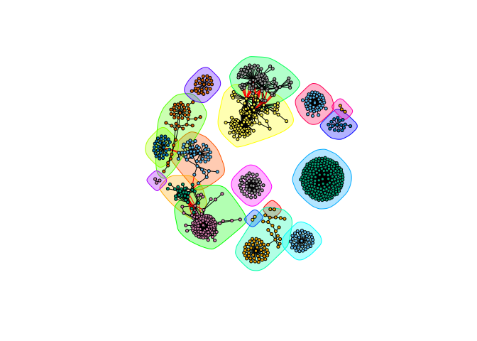
Extract membership information
head(membership(cb))
##  ph_1061  ph_1258  ph_3164  ph_1033 ph_10996 ph_11038
##        1        2        3        4        4        4
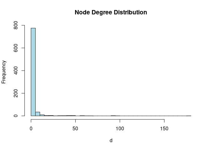
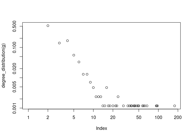
Node degree
# Calculate and plot node degree of our network
d <- degree(g)
hist(d, breaks=30, col="lightblue", main ="Node Degree Distribution")
plot( degree_distribution(g), type="h" )
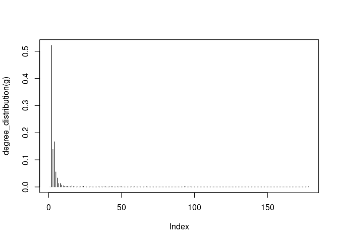
plot(degree_distribution(g), log = 'xy')
## Warning in xy.coords(x, y, xlabel, ylabel, log): 138 y values <= 0 omitted
## from logarithmic plot
Centrality Analaysis
Answer this question: Which nodes are the most important and why???
First method: PageRank
pr <- page_rank(g)
head(pr$vector)
##      ph_1061      ph_1258      ph_3164      ph_1033     ph_10996
## 0.0011834320 0.0011599483 0.0019042088 0.0005788564 0.0005769663
##     ph_11038
## 0.0005745460
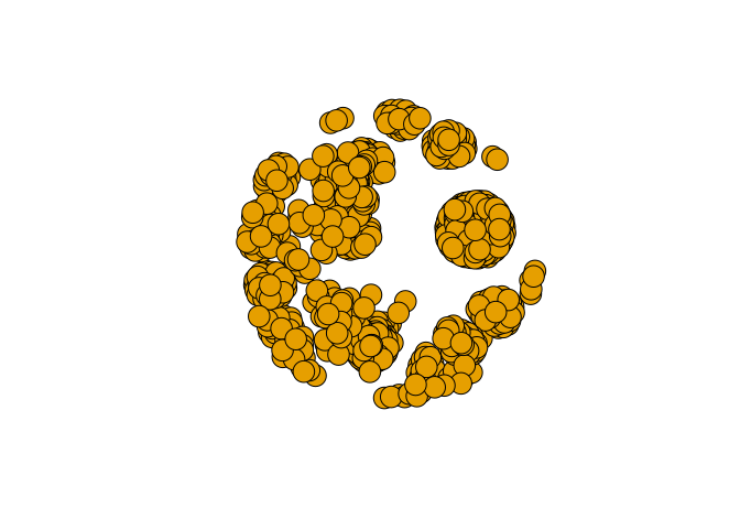
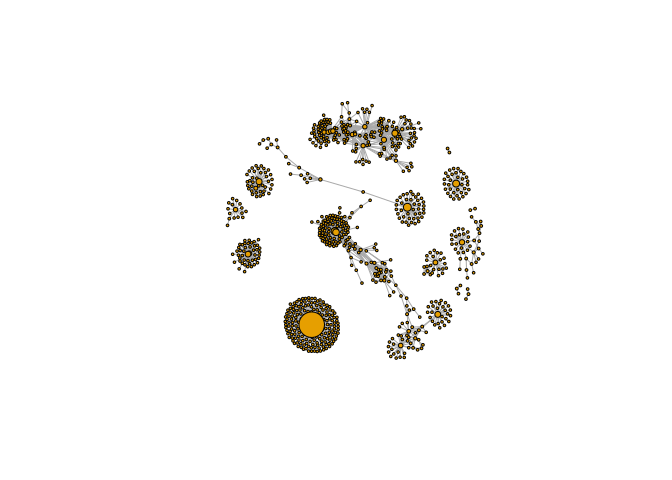
Plot graph with nodes scaled by page rank score
# Make a size vector btwn 2 and 20 for node plotting size

v.size <- BBmisc::normalize(pr$vector, range=c(2,20), method="range")
plot(g, vertex.size=v.size, vertex.label=NA)
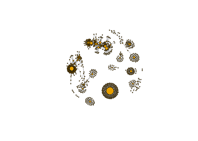
Second method: node degree
v.size <- BBmisc::normalize(d, range=c(2,20), method="range")
plot(g, vertex.size=v.size, vertex.label=NA)
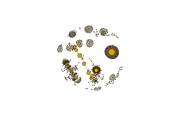
Third method: betweenness
b <- betweenness(g)
v.size <- BBmisc::normalize(b, range=c(2,20), method="range")
plot(g, vertex.size=v.size, vertex.label=NA)
Read taxonomic classification for network annotation
phage_id_affiliation <- read.delim("./data/phage_ids_with_affiliation.tsv")
head(phage_id_affiliation)
##   first_sheet.Phage_id first_sheet.Phage_id_network phage_affiliation
## 1        109DCM_115804                       ph_775              <NA>
## 2        109DCM_115804                       ph_775              <NA>
## 3        109DCM_115804                       ph_775              <NA>
## 4        109DCM_115804                       ph_775              <NA>
## 5        109DCM_115804                       ph_775              <NA>
## 6        109DCM_115804                       ph_775              <NA>
##   Domain DNA_or_RNA Tax_order Tax_subfamily Tax_family Tax_genus
## 1   <NA>       <NA>      <NA>          <NA>       <NA>      <NA>
## 2   <NA>       <NA>      <NA>          <NA>       <NA>      <NA>
## 3   <NA>       <NA>      <NA>          <NA>       <NA>      <NA>
## 4   <NA>       <NA>      <NA>          <NA>       <NA>      <NA>
## 5   <NA>       <NA>      <NA>          <NA>       <NA>      <NA>
## 6   <NA>       <NA>      <NA>          <NA>       <NA>      <NA>
##   Tax_species
## 1        <NA>
## 2        <NA>
## 3        <NA>
## 4        <NA>
## 5        <NA>
## 6        <NA>
bac_id_affi <- read.delim("./data/prok_tax_from_silva.tsv", stringsAsFactors = FALSE)
head(bac_id_affi)
##    Accession_ID  Kingdom         Phylum          Class             Order
## 1 AACY020068177 Bacteria    Chloroflexi   SAR202 clade marine metagenome
## 2 AACY020125842  Archaea  Euryarchaeota Thermoplasmata Thermoplasmatales
## 3 AACY020187844  Archaea  Euryarchaeota Thermoplasmata Thermoplasmatales
## 4 AACY020105546 Bacteria Actinobacteria Actinobacteria             PeM15
## 5 AACY020281370  Archaea  Euryarchaeota Thermoplasmata Thermoplasmatales
## 6 AACY020147130  Archaea  Euryarchaeota Thermoplasmata Thermoplasmatales
##              Family             Genus Species
## 1              <NA>              <NA>    <NA>
## 2   Marine Group II marine metagenome    <NA>
## 3   Marine Group II marine metagenome    <NA>
## 4 marine metagenome              <NA>    <NA>
## 5   Marine Group II marine metagenome    <NA>
## 6   Marine Group II marine metagenome    <NA>
## Extract out our vertex names
genenet.nodes <- as.data.frame(vertex.attributes(g), stringsAsFactors=FALSE)
head(genenet.nodes)
##       name
## 1  ph_1061
## 2  ph_1258
## 3  ph_3164
## 4  ph_1033
## 5 ph_10996
## 6 ph_11038
How many phage entries do we have?
sum(grepl('ph_', genenet.nodes$name))
## [1] 764
Merge annotation data with phylogenetic data…
# We dont need all annotation data so lets make a reduced table 'z' for merging
z <- bac_id_affi[,c("Accession_ID", "Kingdom", "Phylum", "Class")]
n <- merge(genenet.nodes, z, by.x="name", by.y="Accession_ID", all.x=TRUE)
head(n)
##            name  Kingdom          Phylum               Class
## 1 AACY020068177 Bacteria     Chloroflexi        SAR202 clade
## 2 AACY020207233 Bacteria Deferribacteres     Deferribacteres
## 3 AACY020255495 Bacteria  Proteobacteria Gammaproteobacteria
## 4 AACY020288370 Bacteria  Actinobacteria      Acidimicrobiia
## 5 AACY020396101 Bacteria  Actinobacteria      Acidimicrobiia
## 6 AACY020398456 Bacteria  Proteobacteria Gammaproteobacteria
# Again we only need a subset of `phage_id_affiliation` for our purposes
y <- phage_id_affiliation[, c("first_sheet.Phage_id_network", "phage_affiliation","Tax_order", "Tax_subfamily")]

# Add the little phage annotation that we have
x <- merge(x=n, y=y, by.x="name", by.y="first_sheet.Phage_id_network", all.x=TRUE)

## Remove duplicates from multiple matches
x <- x[!duplicated( (x$name) ),]
head(x)
##            name  Kingdom          Phylum               Class
## 1 AACY020068177 Bacteria     Chloroflexi        SAR202 clade
## 2 AACY020207233 Bacteria Deferribacteres     Deferribacteres
## 3 AACY020255495 Bacteria  Proteobacteria Gammaproteobacteria
## 4 AACY020288370 Bacteria  Actinobacteria      Acidimicrobiia
## 5 AACY020396101 Bacteria  Actinobacteria      Acidimicrobiia
## 6 AACY020398456 Bacteria  Proteobacteria Gammaproteobacteria
##   phage_affiliation Tax_order Tax_subfamily
## 1              <NA>      <NA>          <NA>
## 2              <NA>      <NA>          <NA>
## 3              <NA>      <NA>          <NA>
## 4              <NA>      <NA>          <NA>
## 5              <NA>      <NA>          <NA>
## 6              <NA>      <NA>          <NA>
Save the annotation data to the graph nodes..
genenet.nodes <- x
Send network to Cytoscape using RCy3
# delete any existing networks
deleteAllNetworks()
# Set the main nodes colname to the required "id"
colnames(genenet.nodes)[1] <- "id"
Add the network data to edges/nodes and send to cytoscape
genenet.edges <- data.frame(igraph::as_edgelist(g))

# Set the main edges colname to the required "source" and "target"
colnames(genenet.edges) <- c("source","target")

# Add the weight from igraph to a new column...
genenet.edges$Weight <- igraph::edge_attr(g)$weight

# Send as a new network to Cytoscape
createNetworkFromDataFrames(genenet.nodes,genenet.edges,
                            title="Tara_Oceans")
## Loading data...
## Applying default style...
## Applying preferred layout...

## networkSUID
##        7807
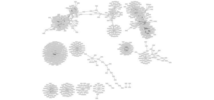
Save a figure of the cytoscape network here…
fig <- exportImage(filename="tara_oceans", type="png", height=350)
## Warning: This file already exists. A Cytoscape popup
##                 will be generated to confirm overwrite.
knitr::include_graphics("./tara_oceans.png")